R in school: the ecologist

The ecology units in science are some of the most memorable lessons, for both staff and pupils. Children love to go out and do science in the real world: explore habitats and organisms under a microscope, suck an aphid into a pooter, sweep the school pond with a net, count the number of daisies on the field … .

Speaking of counting daisies on the field, this is where pupils have to sample an area for various reasons. The interesting question here is where do you begin? As far as the exam boards are concerned, you tell the pupils to randomly place a quadrat in the area in question. But how would a pupil pick a random place, and how random is this?

If you are on your own on a big wide field, closing your eyes, taking a few spins, and throwing the quadrat is good enough fun. When you have a class of 30 pupils, however, aimlessly throwing quadrats is not a good idea.

Supposing your school field is 100 m $\times$ 100 m, you could generate two random numbers for each pupil, ranging from 0 to 100. Placing two tape measures perpendicularly, the pupils can use their numbers as $x$ and $y$ coordinates for where they should place their quadrats.

Here’s how you can generate two random numbers for each pupil.

# Import required packages
library(tidyverse)

# Number of pupils
my_pop <- 30

# Randomly generate two number for each pupil
df <- tibble(
  Name = c(paste0("Pupil ", 1:my_pop)),
  "Across the field in metres" = sample(x = seq(0, 100, 1), size = my_pop, replace = TRUE),
  "Up the field in metres" = sample(x = seq(0, 100, 1), size = my_pop, replace = TRUE)
)

Name

Across the field in metres

Up the field in metres

Pupil 1

49

82

Pupil 2

69

30

Pupil 3

72

67

Pupil 4

19

81

Pupil 5

51

14

Pupil 6

29

41

Pupil 7

34

9

Pupil 8

39

5

Pupil 9

54

21

Pupil 10

29

99

1–10 of 30 rows

Note

Generating true random numbers is incredibly difficult. Since computers use mathematical formulae to generate their random numbers, they are not truly random, but rather pseudo-random. For this article, pseudo-random is fine.

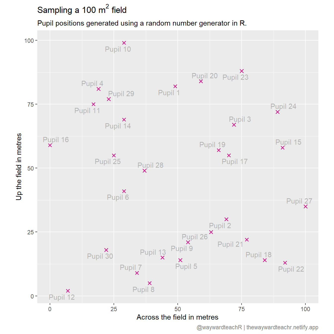
This is perfectly easy to do in Excel, but the following isn’t. Here’s how you can plot a bird’s-eye view of the pupils’ positions:

df |>
  ggplot(aes(x = `Across the field in metres`, y = `Up the field in metres`)) +
  geom_point(shape = 4, stroke = 1, col = "violetred") +
  ggrepel::geom_text_repel(ggplot2::aes(label = Name), col = "grey70") +
  coord_fixed() +
  labs(
    title = expression(paste("Sampling a 100 ", m^2, " field")),
    subtitle = "Pupil positions generated using a random number generator in R."
  )

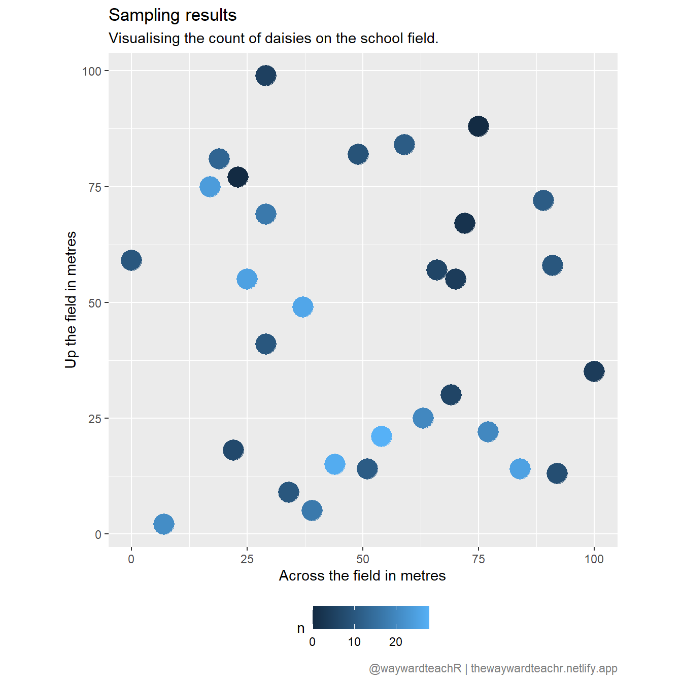
Let’s suppose you collected the pupils’ results and it looks something like this:

Name

Across the field in metres

Up the field in metres

Count of daisies

Pupil 1

49

82

9

Pupil 2

69

30

6

Pupil 3

72

67

2

Pupil 4

19

81

13

Pupil 5

51

14

11

Pupil 6

29

41

10

Pupil 7

34

9

10

Pupil 8

39

5

17

Pupil 9

54

21

28

Pupil 10

29

99

5

1–10 of 30 rows

The beauty of using R is that you can quickly visualise this into something meaningful for the pupils. For very many pupils, tables are notoriously difficult to comprehend. In this case, there is too much data in table-form for anyone to see bigger patterns.

df |>
  ggplot(aes(x = `Across the field in metres`, y = `Up the field in metres`, col = `Count of daisies`)) +
  geom_point(size = 7) +
  coord_fixed() +
  labs(
    x = "Across the field in metres", y = "Up the field in metres",
    title = "Sampling results",
    subtitle = "Visualising the count of daisies on the school field."
  )

Using the {ggdensity} package, you can go one step further and plot a probability density map of the distribution of daisies on the school field.

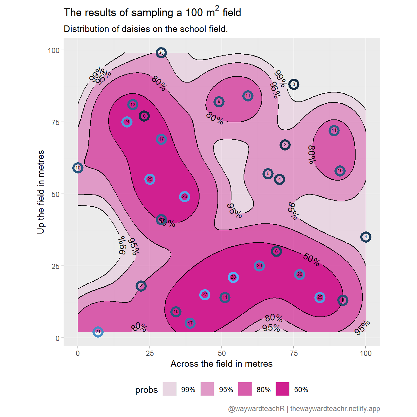
I hope to write more about the {ggdensity} package in a future article. Keep watching.

Corrections

If you spot any mistakes or want to suggest changes, please let me know through the usual channels.