R in school: the AHT – The wayward teachR

It’s a hot and humid day in the office and your mind wanders off to your past. You don’t know why, but it’s been happening quite a lot recently.

You are the child of strict but deeply sincere parents; they were poor, but industrious and managed to spare you the full rigours of poverty only too prevalent in the area in which you grew up. Your parents were ambitious and, determined that you should move your station beyond theirs, they tutored you in the precious little time they had outside of work and managed to get you into the local grammar school …

The deputy headteacher knocks on your door and you duly snap out of your untimely slumber. You have been tasked with assigning target grades for next year’s Y10. Normally, this isn’t a problem, because every school has overpriced software that do these things for SLT. But not this school. This school is poor. Very poor. You are a rising star in the LA and, though you could have gone to any other school for your AHT-ship, you chose this school because it reminded you of the deprivation in which you grew up — something about wanting to help the forgotten poor appealed to you — and because the headteacher and deputy left an impression on you in interview.

You open up your school’s information management system (MIS) and find that there are KS2 scaled scores for each pupil. It looks something like this:

Being one of the few AHTs in the country to have read the DfE’s guidance on secondary accountability measures back-to-back — all 81 pages — you know that there are tables upon tables that match KS2 scaled scores to GCSE attainment in various subjects. You also know that target grades for pupils don’t exist until after the GCSE exams are sat and analysed by government bean counters, but arguing that point is a battle for another day.

On a piece of paper, you quickly jot down the steps you need to take to fulfil your task. You do this before your mind wanders off again.

Obtain KS2 scores for current Y9 (who will be Y10 in September).
Get hold of DfE’s 2022 guide that links KS2 scores to GCSE attainment.
Map Y9 KS2 scores to DfE’s dataset.
Using DfE’s guidance, categorise pupils into H, M, and L prior attainment groups.

The steps appear straightforward enough. You have already done step one. For step two, you turn to page 72 of the DfE’s guidance on secondary accountability measures.

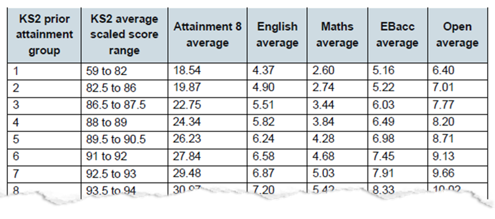
Extract from page 72 of the DfE’s guide.

And then at once it dawns on you: the data tables are in a .pdf document. In order to map your Y9 KS2 scores to GCSE attainment, you need to extract the tables. But how? You tried to copy-paste into Excel, but it doesn’t quite work the way you need it to, and the second column has number and text that need separating. You feel that lump in your throat, knowing that you will have to manually type everything out. In the midst of the heartache, your mind wanders again.

Growing up, your education cost your parents all the little free time they had and the expense of feeding and clothing you; that was a sufficiently large sacrifice to the poor of their generation. Though you were never able to adequately express your thankfulness to them, you are eternally grateful for their love and devotion and unfailing encouragement …

You snap out of it again. You know there must be an easier way to do this.

There is.

It’s called R.

Let’s `R`

Step 2: Use `R` to get DfE’s attainment data into useable form

First, tell R to load the {tidyverse} and {tabulizer} packages. If you don’t have these installed, do so now.

# Install packages
install.packages("tidyverse")
install.packages("remotes")
remotes::install_github(c("ropensci/tabulizerjars", "ropensci/tabulizer"),
                        INSTALL_opts = "--no-multiarch",
                        force = TRUE)

Load the packages and tell R where the DfE’s guidance document is saved.

# Load packages
library(tidyverse)
library(tabulizer)

# Define directory where pdf is saved
my_dir <- "C:/Blah/Blah/Blah/"

# Get pdf
my_pdf <- paste0(my_dir, "Secondary_accountability_measures_2023-04.pdf")

Using the extract_tables() function from the {tabulizer} package, we can extract the prior attainment data from the .pdf into a list of dataframes. The bind_rows() function is used to collapse the list into a single dataframe.

# Import table from pdf
df <- extract_tables(my_pdf, pages = 72, guess = FALSE, output = "data.frame")

# Collapse list
df <- bind_rows(df)

Let’s have a quick glimpse at what the extracted data looks like.

# Glimpse
head(df[[1]])

[1] "each KS2 prior attainment group"                              
[2] "KS2 prior KS2 average"                                        
[3] "Open attainment scaled score Attainment 8 English Maths EBacc"
[4] "average group range average average average average"          
[5] "1 59 to 82 18.54 4.37 2.60 5.16 6.40"                         
[6] "2 82.5 to 86 19.87 4.90 2.74 5.22 7.01"

It looks a bit of a mess and needs tidying up, but it’s all easily doable. From the glimpse, there are two things to realise:

the first four rows are unnecessary;
different columns from page 72 appear to be separated by a space here.

Drop the first four rows and create a new column heading KS2.PAG as follows:

# Drop first four rows
df <- df[-c(1:4), ]

# New column heading
df <- data.frame("KS2.PAG" = df)

Take another quick glimpse.

# Glimpse
head(df)

                                   KS2.PAG
1     1 59 to 82 18.54 4.37 2.60 5.16 6.40
2   2 82.5 to 86 19.87 4.90 2.74 5.22 7.01
3 3 86.5 to 87.5 22.75 5.51 3.44 6.03 7.77
4     4 88 to 89 24.34 5.82 3.84 6.49 8.20
5 5 89.5 to 90.5 26.23 6.24 4.28 6.98 8.71
6     6 91 to 92 27.84 6.58 4.68 7.45 9.13

We can now separate our new KS2.PAG column wherever there are spaces in the dataset.

# Separate columns
df <- df |>
  separate(
    col = KS2.PAG,
    into = c("KS2.PAG", "KS2.Scaled.Min", "To", "KS2.Scaled.Max",
             "A8.Av", "English.Av", "Maths.Av", "Ebacc.Av", "Open.Av"),
    sep = " "
  )

# Glimpse
head(df)

This is almost perfect, but we’re not quite there yet. The extract_tables() function also extracted the page number, 72, and appended it to the end of the dataframe. There is also a To column that we don’t need.

# Glimpse
tail(df)

The easiest way of removing the last row is by using the nrow() function. The nrow() function simply tells you how many rows there are in your dataframe. Given that we want to remove the last row, the number of rows in our dataframe is the last row.

# Drop last row
df <- df[-nrow(df), ]

Take another look using tail(df) to see that the previous last row has been removed.

Let’s now remove the To column.

# Remove "To" column
df$To <- NULL

The other thing that is still wrong with the table is that R thinks everything is a character. You can check this by typing str(df).

# Inspect structure
str(df)

'data.frame':   34 obs. of  8 variables:
 $ KS2.PAG       : chr  "1" "2" "3" "4" ...
 $ KS2.Scaled.Min: chr  "59" "82.5" "86.5" "88" ...
 $ KS2.Scaled.Max: chr  "82" "86" "87.5" "89" ...
 $ A8.Av         : chr  "18.54" "19.87" "22.75" "24.34" ...
 $ English.Av    : chr  "4.37" "4.90" "5.51" "5.82" ...
 $ Maths.Av      : chr  "2.60" "2.74" "3.44" "3.84" ...
 $ Ebacc.Av      : chr  "5.16" "5.22" "6.03" "6.49" ...
 $ Open.Av       : chr  "6.40" "7.01" "7.77" "8.20" ...

You can’t do maths on characters. You need to convert them to numbers. To convert everything to numeric, type

# Convert all columns to numeric
df <- df |>
  mutate(across(.cols = everything(), .fns = as.numeric))

Let’s have a look.

# Inspect structure
str(df)

'data.frame':   34 obs. of  8 variables:
 $ KS2.PAG       : num  1 2 3 4 5 6 7 8 9 10 ...
 $ KS2.Scaled.Min: num  59 82.5 86.5 88 89.5 91 92.5 93.5 94.5 95.5 ...
 $ KS2.Scaled.Max: num  82 86 87.5 89 90.5 92 93 94 95 96 ...
 $ A8.Av         : num  18.5 19.9 22.8 24.3 26.2 ...
 $ English.Av    : num  4.37 4.9 5.51 5.82 6.24 6.58 6.87 7.2 7.48 7.76 ...
 $ Maths.Av      : num  2.6 2.74 3.44 3.84 4.28 4.68 5.03 5.42 5.8 6.12 ...
 $ Ebacc.Av      : num  5.16 5.22 6.03 6.49 6.98 7.45 7.91 8.33 8.77 9.17 ...
 $ Open.Av       : num  6.4 7.01 7.77 8.2 8.71 ...

Okay, that is step two done. Now you have the DfE’s attainment data in a useable format.

Step 3: Use `R` to map Y9 KS2 scores to the DfE dataset.

To accomplish this task, we need to match our Y9 KS2.Scaled.Mean column to the range defined in the DfE’s KS2.Scaled.Min and KS2.Scaled.Max columns. The package {fuzzyjoin} makes this a breeze. Go ahead and install it.

# Install fuzzyjoin
install.packages("fuzzyjoin")

Import the spreadsheet containing your Y9 KS2 scaled scores — the one you exported from your school’s MIS.

# Import your Y9 data into R
df_y9 <- read.csv("my_exported_data.csv")

We will use the fuzzy_inner_join() function to get R to merge our data.

# Load packages
library(fuzzyjoin)

# Join
df_y9 <- fuzzy_inner_join(
  df_y9, df,
  by = c("KS2.Scaled.Mean" = "KS2.Scaled.Min",
         "KS2.Scaled.Mean" = "KS2.Scaled.Max"), 
  match_fun = list(`>=`, `<=`)
)

Let’s take a look to see that it has worked.

# Glimpse
head(df_y9)

Yep. Looks good, but attainment eight (A8) is calculated over 10 subjects; this, therefore, needs dividing by 10 to get the average on a per subject basis. In fact

A8 needs dividing by 10;
English needs dividing by two, because it is counted twice;
Maths needs dividing by two, because it is counted twice;
Ebacc needs dividing by three, because it is counted three times;
Open needs dividing by three, because it is counted three times.

# Compute attainment per subject
df_y9 <- df_y9 |>
  mutate(A8.Av = A8.Av / 10,
         English.Av = English.Av / 2,
         Maths.Av = Maths.Av / 2,
         Ebacc.Av = Ebacc.Av / 3,
         Open.Av = Open.Av / 3)

Let’s take another look to see that it has worked.

# Glimpse
head(df_y9)

Perfect. Pupil 3 has a KS2 scaled mean of 91 and his average GCSE attainment target is, therefore, 2.784. His English target is 3.29, and his maths target is 2.34.

That’s step three done.

Step 4: Use `R` to categorise pupils into H, M, and L prior attainment groups.

On page 26 of the DfE’s guidance on secondary accountability measures, there is a table table defines H, M, and L prior attainment group boundaries.

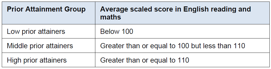
Extract from page 26 of the DfE’s guide.

Knowing this, we can use the ifelse() function to encode this information into a new column called PAG (prior attainment group).

# Encode H, M, and L
df_y9 <- df_y9 |>
  mutate(PAG = ifelse(KS2.Scaled.Mean < 100, "L",
                      ifelse(KS2.Scaled.Mean >= 110, "H", "M")))

Let’s take a final glance.

# Glimpse
head(df_y9)

There it is. You have successfully assigned target grades to each pupil and categorised the pupils into H, M, and L prior attainment groups.

Epilogue

Just as you were about to feel proud of what you had done, your mind zones out again.

Being what was called a clever boy, after grammar school you proceeded to university where you immersed yourself in abstract science and mathematics. You never talked about your background in your new circle and always found a way to change the topic whenever it was brought up in conversation. You read voraciously and dedicated all your time to your studies and, in due course, you won a scholarship for post-graduate studies where a chance encounter would be the turning point in your life. In spite of the sacrifices your parents’ generation had made, you cannot escape the realisation that the poor are becoming poorer still …

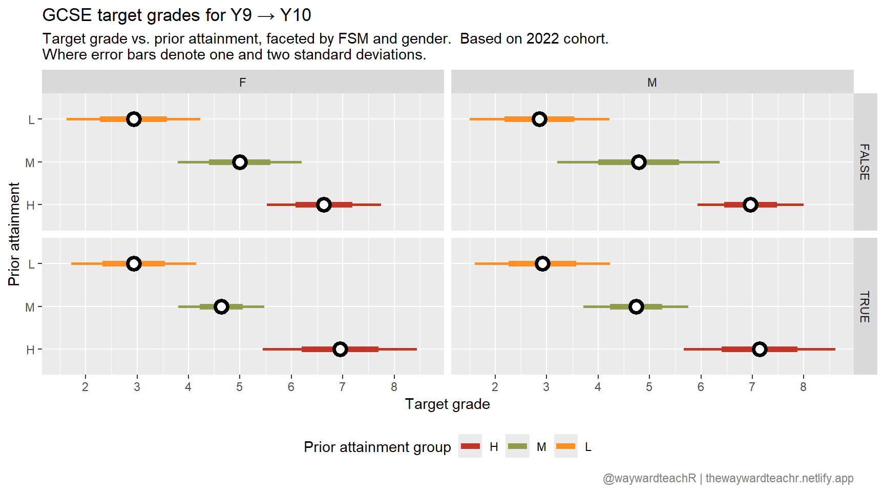
The hazy fog surrounding your mind lifts for a moment and you want to know the general distribution of target grades.

Using the group_by() function, you calculate aggregated statistics based on PAG, gender, and FSM eligibility.

# Compute summary stats
df_y9 |>
  group_by(PAG, Gender, FSM) |>
  summarise(n = n(), Mean = mean(A8.Av), StDev = sd(A8.Av), .groups = "drop") |>
  mutate(StE = StDev / sqrt(n))

Tables are an eye-sore, so you visualise the information instead.

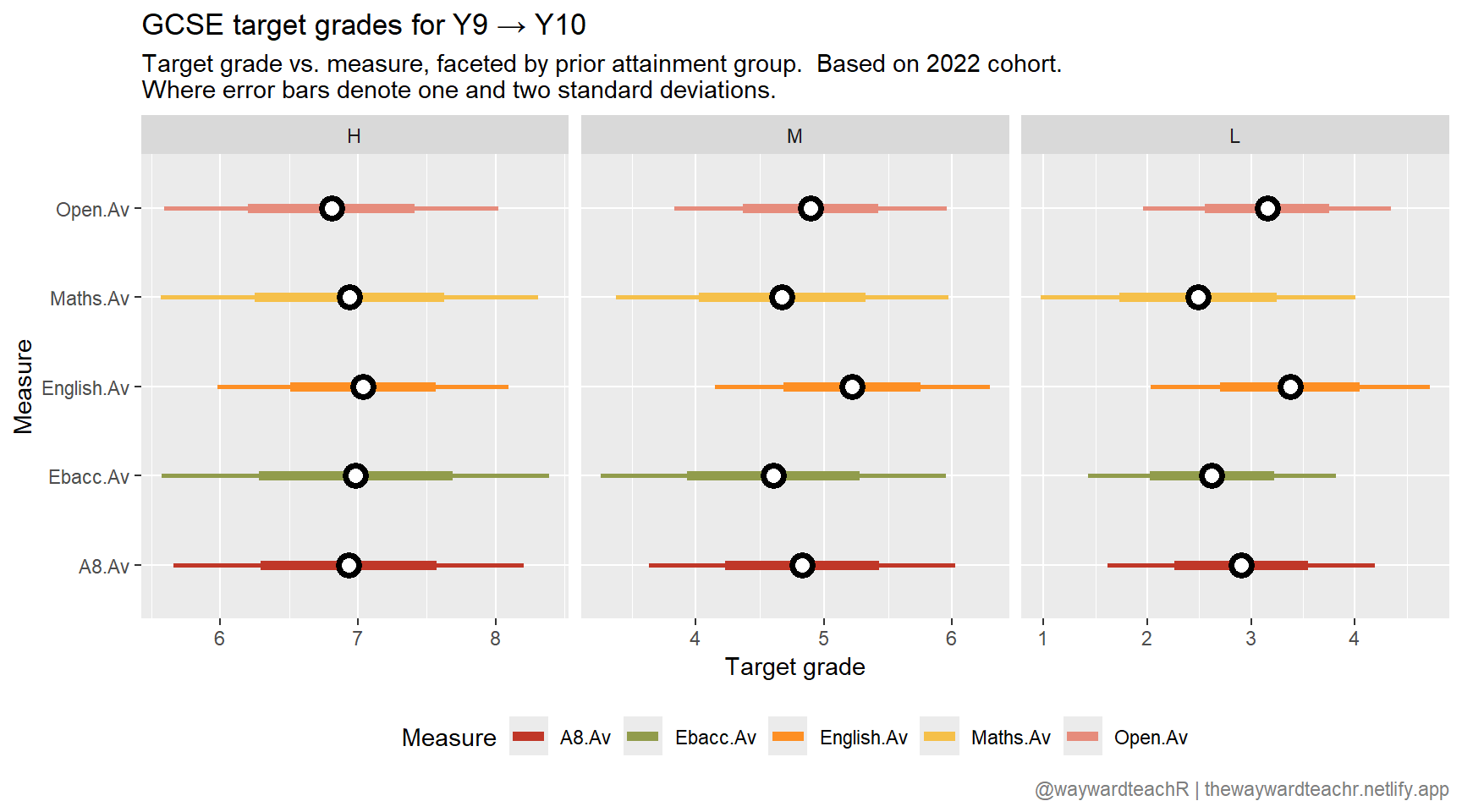
Based on the 2022 cohort, it looks like a slightly higher attainment is needed in English.

How to create plots like this will be posted separately in a future article. Keep watching.

Corrections

If you spot any mistakes or want to suggest changes, please let me know through the usual channels.

Citation

BibTeX citation:

@online{teachr2023,
  author = {teachR, wayward},
  title = {R in School: The {AHT}},
  date = {2023-08-12},
  url = {https://thewaywardteachr.netlify.app/posts/2023-08-12-r-in-school-aht/r-in-school-aht.html},
  langid = {en}
}

For attribution, please cite this work as:

teachR, wayward. 2023. “R in School: The AHT.” August 12, 2023. https://thewaywardteachr.netlify.app/posts/2023-08-12-r-in-school-aht/r-in-school-aht.html.

Let’s R

Step 2: Use R to get DfE’s attainment data into useable form

Step 3: Use R to map Y9 KS2 scores to the DfE dataset.

Step 4: Use R to categorise pupils into H, M, and L prior attainment groups.