R functions

Functions are the meat and potatoes of R. That is no surprise, given that R is a functional programming language.

What is a function?

A function is exactly what you learned in high school maths: a magic box that takes an input and produces an output. Below is a function box called A. The input is 3 and the output is 6.

$$3⟶\left[\begin{array}{c}\mathrm{A}\end{array}\right]⟶6$$

A is a function box because it took the number 3, did something to it, and turned it into 6. ¹

What might be happening inside the function box A? Without further information, it’s difficult to be sure. Here’s a possible solution:

$$3⟶\left[\begin{array}{c}\times 2\end{array}\right]⟶6$$

Writing functions in R

Example 1

Writing functions in R is straightforward. Using our example above, let’s write a function called box_a.

box_a <- function(x) {
  x * 2
}

Our function takes any number, $x$, and multiplies it by 2. Let’s try it out on 3.

box_a(x = 3)

[1] 6

It works!

Given that our function has only one argument ($x$), we don’t even need to write x =.

box_a(3)

[1] 6

Example 2

Let’s write a function to calculate the area of a circle, which takes the equation

$$A=\pi r^2$$

What we want to do is supply $r$, the radius, as an input and have the function output the area, such that

$$r⟶\left[\begin{array}{c}\pi r^2\end{array}\right]⟶A$$

Let’s name the function circle_area.

circle_area <- function(r) {
  pi * r^2
}

Okay. Let’s try it out.

circle_area(7)

[1] 153.938

It works! A circle with a radius 7 has an area 153.938

You might be thinking: I could just do $\pi \times 7^2$ and get the same answer. Yes, but with a function you can do this (and more):

circle_area(r = c(3, 7, 11))

[1]  28.27433 153.93804 380.13271

Braking distance

Let’s take the opportunity to write a function to calculate the braking distance of an object.

Some background for the curious

A moving object has energy associated with its motion. This energy is called kinetic energy. It is defined as

$$E=\frac{1}{2}m{v}^2$$

where $E$ is kinetic energy, $m$ is mass, $v$ is velocity.

In order to slow the object, that moving energy has to be dissipated. In the case of a car, this is done by applying the brakes. In physics-speak, the brakes must do work against the moving car.

$$W=Fx$$

where $W$ is work, $F$ is force, $x$ is distance.

In order to bring the car to a standstill, the amount of work the brakes must do must exactly equal the kinetic energy of the car. In other words

$$W\equiv E$$

This is because of the principle of the conservation of energy.

$$\Rightarrow Fx=\frac{1}{2}m{v}^2$$

Tidying that up a little, we get

$$2Fx=m{v}^2$$

Since we are interested in $x$, the braking distance, rearranging gives

$$x=\frac{m{v}^2}{2F}$$

Newton’s second law of motion tells us that $F=ma$. Substituting that into the equation gives

$$x=\frac{m{v}^2}{2ma}$$

where $a$ is acceleration.

Mass, $m$, cancels out, because it appears as a multiplier and a divisor, leaving us with

$$x=\frac{v^2}{2a}$$

In the case of systems where slowing down (deceleration) is caused by friction, $a=\mu g$. Substituting that into the equation gives

$$x=\frac{v^2}{2\mu g}$$

where $\mu$ is the coefficient of friction, $g$ is the gravitational field strength (which, on Earth is 9.8 N/kg).

Phew!

The function

Let’s name our function braking_distance_x, with arguments v, u, and g.

braking_distance_x <- function(v, u, g = 9.8) {
  (v^2) / (2 * u * g)
}

Using the function for a car travelling at 15 m/s, with a friction coefficient of 0.9 (very dry), and $g$ for Earth, we get

braking_distance_x(v = 15, u = 0.9, g = 9.8)

[1] 12.7551

So, it takes ~13 m of braking to stop a car travelling at 15 m/s.

What’s the point?

The great thing about having a function is that you can loop over it. Taking our braking distance example, wouldn’t it be nice to quickly work out the braking distances for all speeds between 0 m/s and 15 m/s?

Let’s do it.

# Load packages first
library(tidyverse)

# Define a sequence of intervals for our calculations
my_seq <- seq(0, 15, 0.01)

If you want to view the the sequence of numbers, type my_seq in the console. We will input each one of these numbers as $v$ and get our function to output the distance, $x$.

# Apply loop and save results as `my_distances`
my_distances <- sapply(
  my_seq, function(i) braking_distance_x(
    v = i,
    u = 0.9,
    g = 9.8
  )
)

The distances are saved as my_distances. Let’s now turn this into a table (dataframe) we can use more easily.

# Create a dataframe of the results
df <- data.frame(
  v = my_seq,
  x = my_distances
)

Let’s take a quick look.

# Quick glimpse
head(df)

     v            x
1 0.00 0.000000e+00
2 0.01 5.668934e-06
3 0.02 2.267574e-05
4 0.03 5.102041e-05
5 0.04 9.070295e-05
6 0.05 1.417234e-04

That’s great, but the speeds are in metres per second. Let’s convert these to miles per hour instead.

# Create a new column with speeds in mph
df <- df |> mutate(v_mph = v * 2.236936)

Take a look.

# Take a look
head(df)

     v            x      v_mph
1 0.00 0.000000e+00 0.00000000
2 0.01 5.668934e-06 0.02236936
3 0.02 2.267574e-05 0.04473872
4 0.03 5.102041e-05 0.06710808
5 0.04 9.070295e-05 0.08947744
6 0.05 1.417234e-04 0.11184680

While we’re at it, let’s work out the time, $t$, it takes to come to a standstill.

$$v=\frac{x}{t}\Rightarrow t=\frac{x}{v}$$

# Create a new column with times in seconds
df <- df |> mutate(t = x / v)

Take a look.

# Take a look
head(df)

     v            x      v_mph            t
1 0.00 0.000000e+00 0.00000000          NaN
2 0.01 5.668934e-06 0.02236936 0.0005668934
3 0.02 2.267574e-05 0.04473872 0.0011337868
4 0.03 5.102041e-05 0.06710808 0.0017006803
5 0.04 9.070295e-05 0.08947744 0.0022675737
6 0.05 1.417234e-04 0.11184680 0.0028344671

Tables are great for a few rows of data; anything more and you really ought to visualise it.

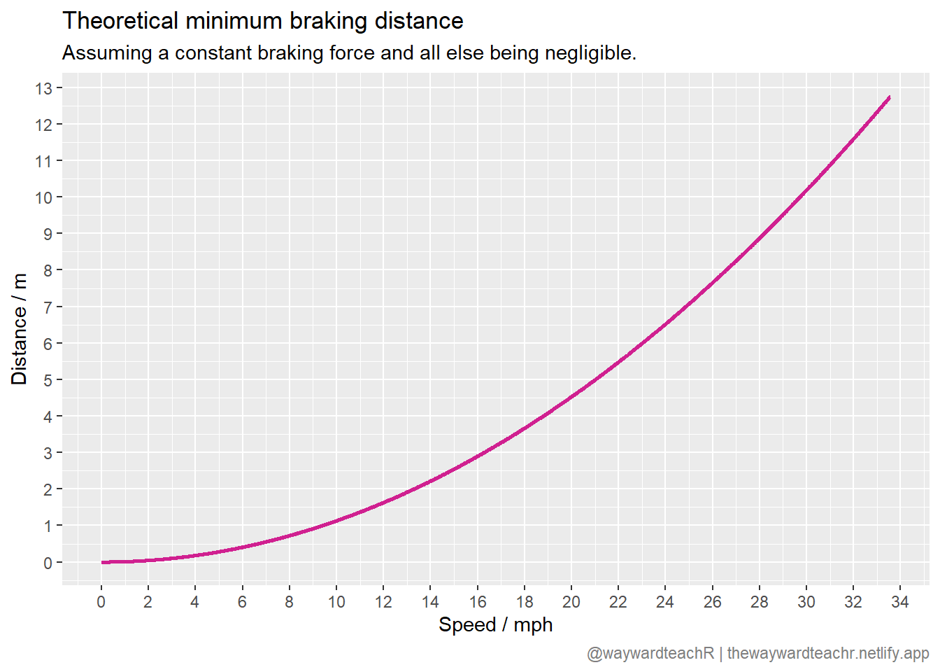
# Create a plot layer-by-layer
# Define data and axes columns
my_plot <- ggplot(data = df, aes(x = v_mph, y = x)) +
  
  # Type of plot
  geom_line(linewidth = 1, col = "violetred") +
  
  # Fine-tune axes scales
  scale_x_continuous(breaks = seq(0, 40, 2)) +
  scale_y_continuous(breaks = seq(0, 15, 1)) +
  
  # Axes titles and labels
  labs(
    x = "Speed / mph", y = "Distance / m",
    title = "Theoretical minimum braking distance",
    subtitle = "Assuming a constant braking force and all else being negligible.",
    caption = "@waywardteachR | thewaywardteachr.netlify.app"
  ) +
  
  # Define text colour for caption
  theme(
    plot.caption = element_text(colour = "grey50")
  )

## View plot
my_plot

If you did everything right, your plot should look something like this:

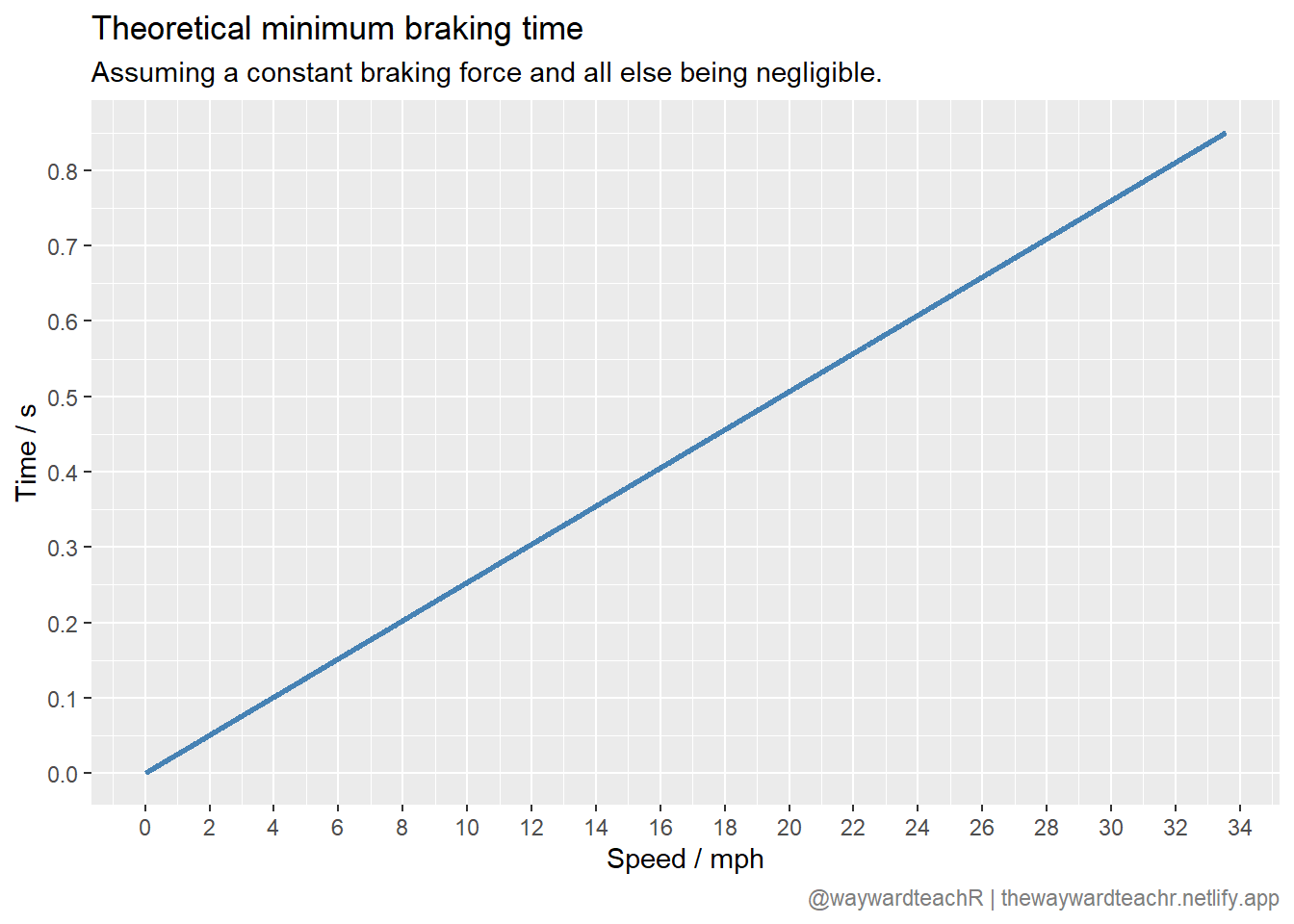
See if you can plot a similar graph for braking time, as opposed to braking distance. Oh, and change the colour, too.

Corrections

If you spot any mistakes or want to suggest changes, please let me know through the usual channels.

Footnotes

1. In maths-speak, did something means it was operated on.