R in school: bayes factors and predicting progress

This is a re-write of an article I wrote more than six years ago on my old blogging site, which went the way of the dodo.

Imagine you are the deputy headteacher of a high school responsible for the curriculum. You like your job and you are pretty good at it, too. You have a meeting coming up with the governors where you are expected give them your best prediction of the school’s progress-eight — in other words, a prediction of the current Y11’s attainment and progress come August.

The governors very much appreciate the hard work and hours you put into the job, but, for the last few years, you have felt like an imposter, because your predictions have been off kilter. You have always relied on the school’s overpriced software for your predictions, which in turn are a reflection of what the classroom teachers have said in the routine data collections. You remind classroom teachers every year not to be too lenient or too harsh in their predictions, but, every year, their figures are off and so are yours.

The meeting with the governors is fast approaching and the only thing on your mind is, prediction: how do I make it better? You are a mathematician by training and, though you have not done any serious maths for nearly two decades, your love for it never died away. You decide today is the day you rekindle that burning desire to do some maths — real maths.

You extract the school’s Y11 data. With a little elbow grease, you find that this year’s Y11s

• are 20% higher prior attainment pupils
• are 52% boys
• are 48% disadvantaged pupils
• are 15% EAL pupils
• have 0% entries for multiple languages
• have 28% triple science entries

You head over to the DfE’s performance tables and extract the 2016-2017 dataset. It is incredibly messy, but, again, with some elbow grease, you manage to sort it. After toiling away into the night, you declare: a school with

• 20% higher ability pupils
• 52% boys
• 48% disadvantaged pupils
• 15% EAL pupils
• 0% multiple language entries
• 28% triple science entries

will end up with a mean progress of -0.29 in 2018.

Wait. What?! How?

Okay, let us rewind a little bit. In the real world, you would not use the DfE’s dataset, but rather your school’s own data going back as far as possible. I am not a teacher and so I do not have access to real school data; thus, my reliance on the DfE for example’s sake.

The primary point of this article is that prior data can be used to predict future outcomes, given true correlations and all else being equal.¹

If you want to follow along with the this article, you will need to have R installed and know how to use it. You will also need the same dataset I used, which was the 2016-2017 data from the DfE’s performance tables. I have a clean version for download here.

I kept the column headings as they were from the DfE; so, if you did not read the DfE’s metadata jargon

• P8MEA = progress 8 measure;
• PTPRIORHI = percentage of pupils at the end of key stage 4 with high prior attainment at the end of key stage 2;
• PBPUP = percentage of pupils at the end of key stage 4 who are boys;
• PTFSM6CLA1A = percentage of pupils at the end of key stage 4 who are disadvantaged;
• PTEALGRP2 = percentage of pupils at the end of key stage 4 with English as additional language (EAL);
• PTmultiLan_E = percentage of pupils entering more than one language;
• PTtripleSci_E = percentage of pupils entering biology, chemistry and physics.

In addition, I removed special schools and schools with missing data in any of the retained columns (the DfE suppress data for various reasons).

P8MEA is what we are hoping to predict. It is the dependent variable. In stats-speak it is also called the regressand. The other six are our independent variables. In stats-speak they are often called regressors.

Choice of regressors

There are over 400 columns of information recorded by the DfE for a school. Some are collected, most are calculated. These include things like school name, establishment number, progress 8 measure for boys and girls, various upper and lower confidence intervals, etc. The choice of the six regressors in this study over the 400+ was based purely on wanting to demonstrate a concept for this article.

Linear regression

Without being mathematically rigorous, a regression line is simply a line of best fit that is used to predict the outcome of a dependent variable. The simplest form is linear regression, which is defined by the straight-line equation — the same straight-line equation you learn in high school. ²

Mathematically, the regression of a random variable $Y$ on a random variable $X$ is given as

$$E(Y\mid X=x)$$

This is the expected value of $Y$ when $X$ takes a specific value $x$. The regression of $Y$ on $X$ is linear if

$$E(Y\mid X=x)={\beta }_0+{\beta }_{1}x$$

where ${\beta }_0$ and ${\beta }_1$ determine the intercept and the slope of a specific straight line, respectively.

This is a perfect mathematical model. In reality, though, the model is unable to fully represent the actual relationship between the independent variable and the dependent variable; to take that into account, we include an error term, $ϵ$, in our equation. The assumption is that this error is random, it does not depend on $x$, it has $0$ mean and constant variance, and it takes the form of a gaussian distribution. ³

$$Y={\beta }_0+{\beta }_{1}x+ϵ$$

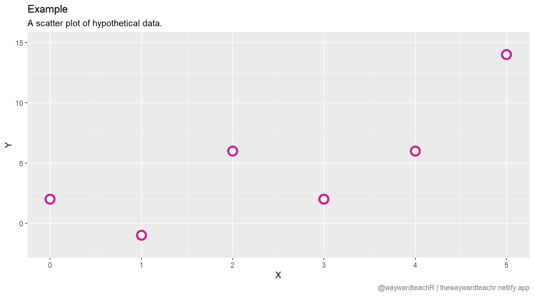
As an example, let’s plot a set of hypothetical data.

# Generate hypothetical data
df_hypothetical <- data.frame(
  x = seq(0, 5, 1),
  y = c(2, -1, 6, 2, 6, 14)
)

# Import package
library(ggplot2)

# Plot hypothetical data
df_hypothetical |>
  ggplot(aes(x = x, y = y)) +
  geom_point(shape = 21, stroke = 2, size = 4, col = "violetred", fill = "white") +
  scale_y_continuous(limits = c(-2, 15), breaks = seq(-5, 20, 5)) +
  scale_size(guide = "none") +
  labs(x = "X", y = "Y",
       title = paste0("Example"),
       subtitle = "A scatter plot of hypothetical data.",
       caption = my_caption) +
  theme(
    plot.caption = element_text(colour = "grey50")
  )

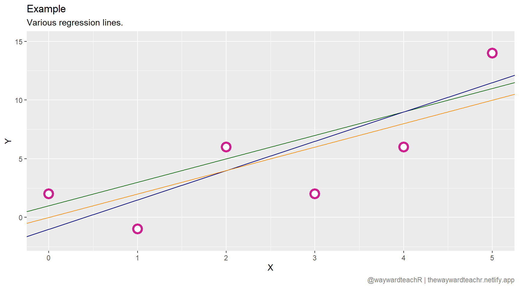
There is a clear correlation between $X$ and $Y$. To predict a possible $\hat{y}$ for a given $x$, we need to draw a regression line that best fits the data. But how? There are an infinite number of lines that can be drawn; three are given in the plot below.

How do we decide on the most appropriate regression line? In order for the regression model to be effective in predicting outcomes, the idea is to minimise the difference between the actual value of $y_i$ and the predicted value of ${\hat{y}}_i$. This difference is called the residual, ${\widehat{ϵ}}_i$.

$${\widehat{ϵ}}_i=y_i-{\hat{y}}_i$$

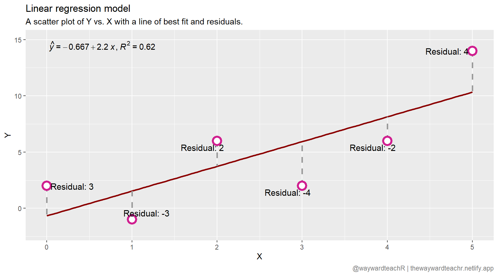
A commonly used technique is the least squares, or residual sum of squares (RSS) method.

$$\mathrm{RSS}=\sum _{i=1}^n{\widehat{ϵ}}_i^2=\sum _{i=1}^n(y_i-{\hat{y}}_i{)}^2=\sum _{i=1}^n(y_i-b_0-b_1{x}_i{)}^2$$

What this does is select a $b_0$ and $b_1$ that minimises the sum of the squared residuals to give us a usable equation to predict the outcome of a dependent variable.

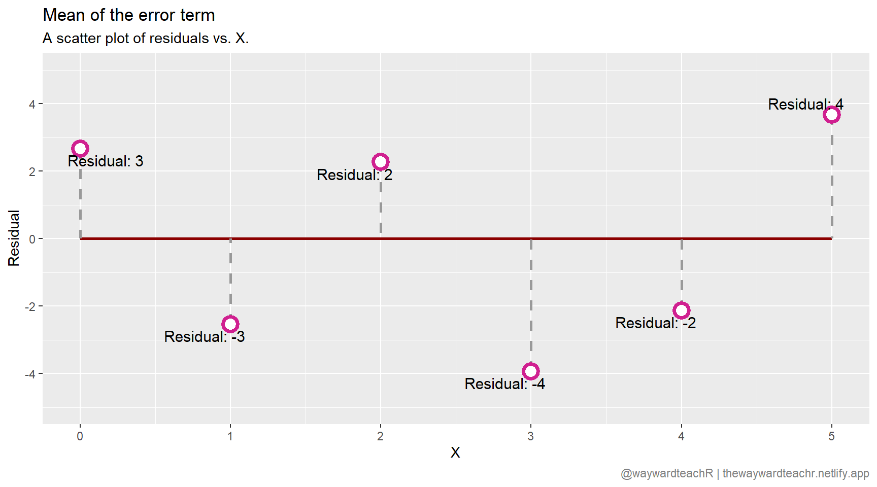
Note that none of the data points fall on the regression line itself, indicating that there are other factors that influence $Y$ other than $X$. This is what the error term encapsulates: the difference between the expected value of ${\hat{y}}_i$ at a particular $x$ and the $y_i$ that was actually observed. That the mean of the error term is $0$ is visually demonstrated in the next plot.

That is great, but how do I extract the equation for the line to start making predictions? Here is how.

# Define linear regression model
linear_model <- lm(y ~ x, data = df_hypothetical)

# View model
linear_model

Call:
lm(formula = y ~ x, data = df_hypothetical)

Coefficients:
(Intercept)            x  
    -0.6667       2.2000  

This tells us that ${\beta }_0=-0.6667$ and ${\beta }_1=2.2$. We now have an equation that should give us the least error in our predictions, given the circumstances.

$$\hat{y}=-0.6667+2.2x$$

To predict a possible $\hat{y}$ for a given $x$, all you have to do is substitute it into the equation above. Let’s predict the value of $\hat{y}$ when $x=6$:

$$\hat{y}=-0.6667+(2.2\times 6)=12.5$$

In R, it is simply

predict(linear_model, data.frame(x = 6), interval = "prediction")

       fit       lwr      upr
1 12.53333 -1.161294 26.22796

lwr and upr are lower and upper 95% confidence intervals.

Simple linear regression

On to our actual data: let us import my clean 2016-2017 dataset into R.

# Import dataset
id_doc <- "1QE4r7QM9GJf9uYgUeY3JOHHELhAb69Wx"
df <- read.csv(sprintf("https://docs.google.com/uc?id=%s&export=download", id_doc))

# Drop school names
df$SCHNAME <- NULL

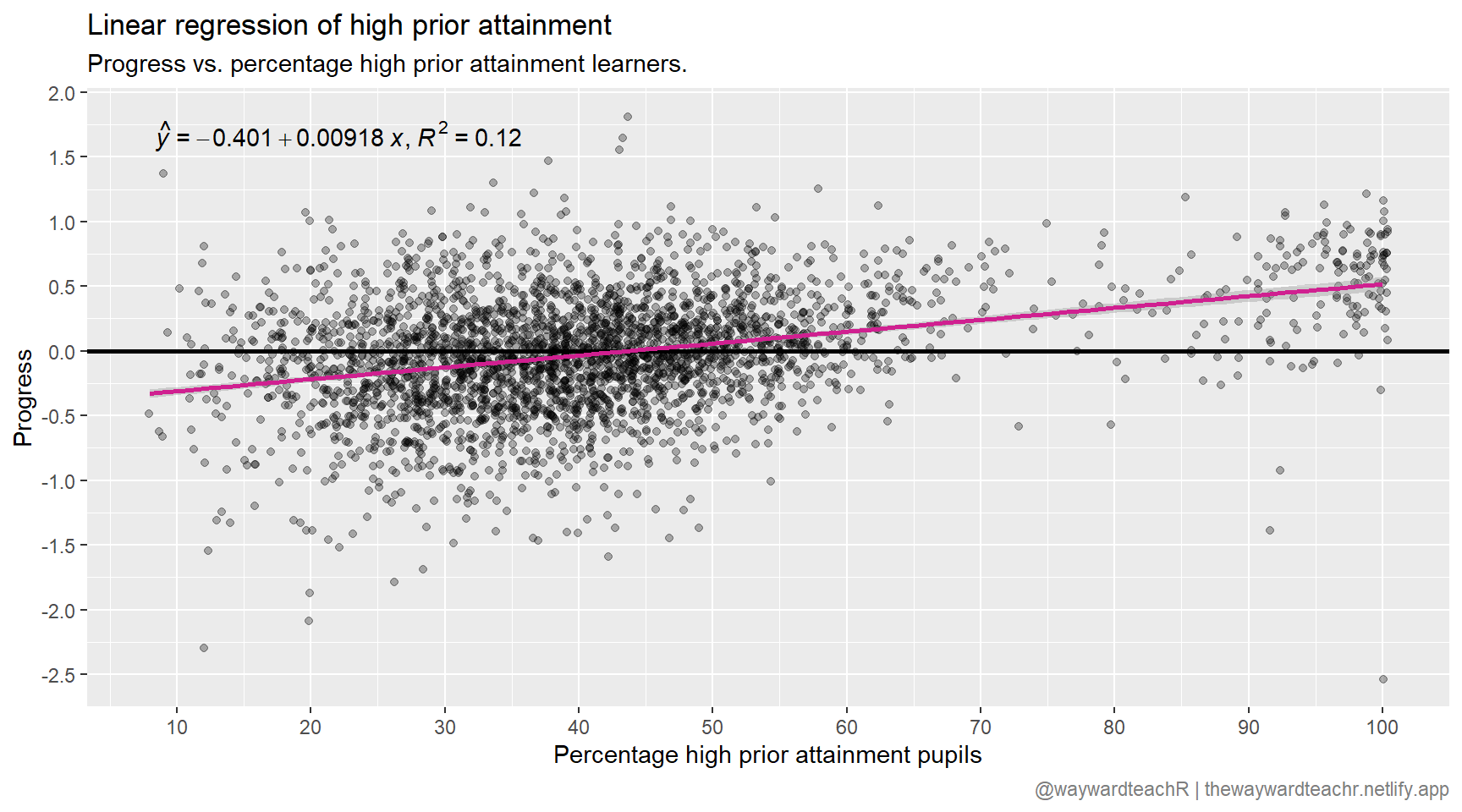
Plotting mean progress against percentage of high prior attainment learners in a school, we find the following picture:

# Import package
library(ggplot2)
library(ggpmisc)

# Plot
df |>
  ggplot(aes(x = PTPRIORHI, y = P8MEA)) +
  geom_hline(yintercept = 0, size = 1, col = "black") +
  geom_jitter(alpha = 0.3) +
  stat_poly_eq(
    formula = y ~ x,
    eq.with.lhs = "italic(hat(y))~`=`~",
    aes(label = paste(..eq.label.., ..rr.label.., sep = "*plain(\",\")~")),
    parse = TRUE
  ) +
  geom_smooth(method = "lm", col = "violetred") +
  scale_y_continuous(limits = c(), breaks = seq(-5, 5, 0.5)) +
  scale_x_continuous(limits = c(), breaks = seq(0, 100, 10)) +
  labs(
    x = "Percentage high prior attainment pupils", y = "Progress",
    title = "Linear regression of high prior attainment",
    subtitle = "Progress vs. percentage high prior attainment learners.",
    caption = my_caption
  ) +
  theme(
    plot.caption = element_text(colour = "grey50")
  )

The $R^2$ value suggests 12% of the variation in progress is explained by the percentage of high prior attainment learners. This tells us that there are other factors at play that have not been accounted for. If I had used only the percentage of high prior attainment learners to predict progress at the beginning of this article, I would have arrived at $-0.22$.

$$\hat{y}=-0.401+(0.00918\times 20)=-0.22$$

A prediction of this sort is known as simple linear regression. This is because we only considered one regressor. It is possible to take more than one regressor into account. First, though, let us ask ourselves: of the six regressors, which ones are significant predictors of a school’s progress? We can find out by typing the following into R:

summary(lm(P8MEA ~ ., data = df))

Call:
lm(formula = P8MEA ~ ., data = df)

Residuals:
     Min       1Q   Median       3Q      Max 
-2.90145 -0.21004  0.00827  0.22109  1.65956 

Coefficients:
                Estimate Std. Error t value Pr(>|t|)    
(Intercept)    0.0917646  0.0390679   2.349   0.0189 *  
PTPRIORHI      0.0032851  0.0006444   5.098 3.65e-07 ***
PBPUP         -0.0043141  0.0003642 -11.845  < 2e-16 ***
PTFSM6CLA1A   -0.0085118  0.0005997 -14.193  < 2e-16 ***
PTEALGRP2      0.0090418  0.0004020  22.493  < 2e-16 ***
PTmultiLan_E   0.0058236  0.0010256   5.678 1.49e-08 ***
PTtripleSci_E  0.0016869  0.0004077   4.138 3.60e-05 ***
---
Signif. codes:  0 '***' 0.001 '**' 0.01 '*' 0.05 '.' 0.1 ' ' 1

Residual standard error: 0.377 on 3112 degrees of freedom
Multiple R-squared:  0.3118,    Adjusted R-squared:  0.3105 
F-statistic:   235 on 6 and 3112 DF,  p-value: < 2.2e-16

It turns out, all six regressors are significant (indicated by the three asterisks; more information can be found over here). This presents us with a problem, because with six regressors there are 63 possible combinations to check through ($2^n-1$). And how would we go about assessing the merits of one combination over another?

This is where bayes factors can help.

Bayes factors

Bayes factors allows us to compare all possible models containing combinations of these regressors; for instance, it may be that a combination of the number of disadvantaged pupils and number of EAL pupils is a better predictor of progress than percentage high prior attainment pupils alone.

There is a package on CRAN called {BayesFactor} that is very good at quickly comparing such models. To install it, type

# Install package
install.packages("BayesFactor")

followed by

# Import package
library(BayesFactor)

# Compute bayes linear regression
bayesian_lr <- regressionBF(P8MEA ~ ., data = df)

You will get a print out of the merits of all 63 combinations. The top seven are listed below.

head(bayesian_lr, n = 7)

Bayes factor analysis
--------------
[1] PTPRIORHI + PBPUP + PTFSM6CLA1A + PTEALGRP2 + PTmultiLan_E + PTtripleSci_E : 1.154918e+244 ±0%
[2] PTPRIORHI + PBPUP + PTFSM6CLA1A + PTEALGRP2 + PTmultiLan_E                 : 4.186979e+241 ±0%
[3] PBPUP + PTFSM6CLA1A + PTEALGRP2 + PTmultiLan_E + PTtripleSci_E             : 5.204965e+239 ±0%
[4] PTPRIORHI + PBPUP + PTFSM6CLA1A + PTEALGRP2 + PTtripleSci_E                : 2.371135e+238 ±0%
[5] PTPRIORHI + PBPUP + PTFSM6CLA1A + PTEALGRP2                                : 3.352253e+235 ±0.01%
[6] PBPUP + PTFSM6CLA1A + PTEALGRP2 + PTmultiLan_E                             : 2.600601e+229 ±0.01%
[7] PBPUP + PTFSM6CLA1A + PTEALGRP2 + PTtripleSci_E                            : 2.455562e+227 ±0.01%

Against denominator:
  Intercept only 
---
Bayes factor type: BFlinearModel, JZS

According to the analysis, a combination of all six regressors is the best — in fact, it is ${10}^{161}$ times better than just considering the percentage of high prior attainment pupils (this is not apparent from the print out above).

Now that we have identified the best model for predicting progress using bayes factors, we can adjust our simple linear regression model to include a combination of all six regressors. Our linear regression model becomes

lm(P8MEA ~ PTPRIORHI + PBPUP + PTFSM6CLA1A + PTEALGRP2 + PTmultiLan_E + PTtripleSci_E, data = df)

Call:
lm(formula = P8MEA ~ PTPRIORHI + PBPUP + PTFSM6CLA1A + PTEALGRP2 + 
    PTmultiLan_E + PTtripleSci_E, data = df)

Coefficients:
  (Intercept)      PTPRIORHI          PBPUP    PTFSM6CLA1A      PTEALGRP2  
     0.091765       0.003285      -0.004314      -0.008512       0.009042  
 PTmultiLan_E  PTtripleSci_E  
     0.005824       0.001687  

This is now a multiple linear regression model, because multiple regressors are taken into account.

Using R’s predict function we can plug in the values from the beginning of this article into our new model and arrive at a calculated prediction. To do that, we first need to create a dataframe containing the values for our regressors.

# Posterior values
df_regressors <- data.frame(
  PTPRIORHI = 20,
  PBPUP = 52,
  PTFSM6CLA1A = 48,
  PTEALGRP2 = 15,
  PTmultiLan_E = 0,
  PTtripleSci_E = 28
)

Let us also define our multiple linear regression model.

# Multiple linear regression model
df_mlr <- lm(P8MEA ~ PTPRIORHI + PBPUP + PTFSM6CLA1A + PTEALGRP2 + PTmultiLan_E + PTtripleSci_E, data = df)

Finally … predict.

# Predict based on posterior values
bayesian_model <- predict(df_mlr, df_regressors, interval = "prediction")
bayesian_model

         fit       lwr       upr
1 -0.2925719 -1.032371 0.4472271

There you have it: a progress prediction of $-0.29\pm 0.74$ at 95% confidence.

Conclusion

Before we conclude, there is a well-known weakness of regression modelling based on observational data, called spurious correlation. This is where an observed association between two variables may be because both are related to a third variable that has been omitted from the regression model. Quoting Sheather, A Modern Approach to Regression with R (which quotes Stigler):

… Pearson studied measurements of a large collection of skulls from the Paris Catacombs, with the goal of understanding the interrelationships among the measurements. For each skull, his assistant measured the length and the breadth, and computed […] the correlation coefficient between these measures […]. The correlation […] turned out to be significantly greater than zero […] but […] the discovery was deflated by his noticing that if the skulls were divided into male and female, the correlation disappeared. Pearson recognized the general nature of this phenomenon and brought it to the attention of the world. When two measurements are correlated, this may be because they are both related to a third factor that has been omitted from the analysis. In Pearson’s case, skull length and skull breadth were essentially uncorrelated if the factor “sex” were incorporated in the analysis.

Moral of the story: omitted variables are very important and must be considered. Similarly, the choice of regressors is just as important. This article played fast and loose with many established practices in statistics in order to demonstrate regression analysis in the prediction of progress.

So … does the predicted progress of -0.29 at the start of the article hold water? In the absence of spurious correlation, yes. Yes, it does.

Further reading

If you want the full maths treatment on regression analysis, you really ought to be reading a book on it. A good place to start that includes some information on R is A Modern Approach to Regression with R by Sheather.

The best statistics book in general is Sheskin’s Handbook of Parametric and Nonparametric Statistical Procedures.

If you want the full treatment in econometrics as a whole, you’re looking for the classic Econometric Analysis of Cross Section and Panel Data by Wooldridge. It’s over a thousand pages of more than you can imagine.

Corrections

If you spot any mistakes or want to suggest changes, please let me know through the usual channels.

Footnotes

1. https://en.wikipedia.org/wiki/Ceteris_paribus

2. You can read more about linear regression over at onlinestatbook.com.

3. The reason for the latter point is to do with the central limit theorem.